Import Data
The dataset we will be working on today will be uber’s NYC September 2014 dataset. You can find the dataset and a bunch more on Kaggle or click here.
Once you have your data, import it, look at the data structure. We’re also going to use the tidyverse package for this tutorial.
str(uber)
 $ Date.Time: Factor w/ 42907 levels "9/1/2014 0:00:00",..: 2 2 4 7 12 13 16 17 33 34 ...
 $ Lat      : num  40.2 40.8 40.8 40.7 40.8 ...
 $ Lon      : num  -74 -74 -74 -74 -73.9 ...
 $ Base     : Factor w/ 5 levels "B02512","B02598",..: 1 1 1 1 1 1 1 1 1 1 ...
Notice that the datetime is a factor and it does not follow the ISO 8601 standard. R likes reading datetimes in this format. The data structure in R is called POSIXct or POSIXlt. We don’t need to get into the details of it but just know that when you run an str() POSIXct or POSIXlt is preferable. You will run into a bunch of problems if it is otherwise.
| Date.Time | Lat | Lon | Base |
|---|---|---|---|
| 9/1/2014 0:01:00 | 40.2201 | -74.0021 | B02512 |
| 9/1/2014 0:01:00 | 40.7500 | -74.0027 | B02512 |
| 9/1/2014 0:03:00 | 40.7559 | -73.9864 | B02512 |
| 9/1/2014 0:06:00 | 40.7450 | -73.9889 | B02512 |
| 9/1/2014 0:11:00 | 40.8145 | -73.9444 | B02512 |
| 9/1/2014 0:12:00 | 40.6735 | -73.9918 | B02512 |
Clean Datetime
There’s a bunch of different ways to clean up datatimes but the method is more or less the same:
- Convert factor to character
uber$Date.Time = as.character(uber$Date.Time)
- Use a datetime function to convert from chr to POSIXct/POSIXlt
uber$Date.Time = strptime(uber$Date.Time, "%m/%d/%Y %H:%M:%S") #base r
parse_date_time(uber$Date.Time, order = 'mdy HMS') #readr package
strptime() is very fast but is not flexible with weird date formats. It will work fine for this dataset. Below is a chart of datetime formats you will encounter and how you should specify your datetime when you convert it in strptime()
Datetime formats
| R Format | Meaning | R Format | Meaning |
|---|---|---|---|
| %a | Abbreviated weekday | %A | Full weekday |
| %b | Abbreviated month | %B | Full month |
| %c | Locale-specific date and time | %d | Decimal date |
| %H | Decimal hours (24 hour) | %I | Decimal hours (12 hour) |
| %j | Decimal day of the year | %m | Decimal month |
| %M | Decimal minute | %p | Locale-specific AM/PM |
| %S | Decimal second | %U | Decimal week of the year (starting on Sunday) |
| %w | Decimal Weekday (0=Sunday) | %W | Decimal week of the year (starting on Monday) |
| %x | Locale-specific Date | %X | Locale-specific Time |
| %y | 2-digit year | %Y | 4-digit year |
| %z | Offset from GMT | %Z | Time zone (character) |
parse_date_time is a more forgiving datetime function. It accepts a wider range of datetime formats and you will not need to use the chart above to specify your datetimes. However, this makes the function a lot slower to work with. If your datetime follows some kind of uniform pattern, strptime() will work just fine.
Aggregate Data
Let’s look at trip volume per day by base.
- Extract date from datetime:
uber$date = substr(uber$Date.Time, 1,10)
- date is now a
chr, convert it toPOSIXlt:uber$date = strptime(uber$date, "%Y-%m-%d")
- Aggregate the data:
table(uber$date,uber$Base)
| Date | B02512 | B02598 | B02617 | B02682 | B02764 |
|---|---|---|---|---|---|
| 2014-09-01 | 638 | 4626 | 7940 | 3677 | 3080 |
| 2014-09-02 | 1188 | 6970 | 11642 | 5729 | 3302 |
| 2014-09-03 | 1284 | 8079 | 13019 | 6462 | 3787 |
| 2014-09-04 | 1513 | 9412 | 15185 | 7670 | 4580 |
| 2014-09-05 | 1808 | 10036 | 16472 | 8660 | 5343 |
| 2014-09-06 | 1580 | 9848 | 15573 | 8132 | 5387 |
| 2014-09-07 | 1124 | 7122 | 11639 | 5983 | 4266 |
| … | … | … | … | … | … |
We might want this to be in a data frame, so we can play around with it.
trips = data.frame(table(uber$date,uber$Base))- Notice that our data is saved in a long format. It’s not as nicely formatted as the chart above. We’ll revisit this later when we graph our data.
trips = spread(trips,Var2,Freq)This reformats our data nicely.
Now our data frame should look something like the chart above but the date is named Var1.
colnames(trips[1]) <- "date" That should fix it!
Graph
Now it’s time to graph. You want your data in a long format like what trips = data.frame(table(uber$date,uber$Base)) gave you. You can just re-run this code or you can use gather() function to bring our data frame back to it’s original state.
graph = gather(trips,'B02512','B02598', 'B02682', 'B02764', 'B02617', key = "Base", value = "Trips")
| date | Base | Trips |
|---|---|---|
| 2014-09-01 | B02512 | 638 |
| 2014-09-02 | B02512 | 1188 |
| 2014-09-03 | B02512 | 1284 |
| 2014-09-04 | B02512 | 1513 |
| 2014-09-05 | B02512 | 1808 |
| 2014-09-06 | B02512 | 1580 |
It looks like our dates are back into factors. No worries, since we’re already in the ISO 8601 format, converting is a breeze.
graph$date = as.POSIXct(as.character(graph$date))
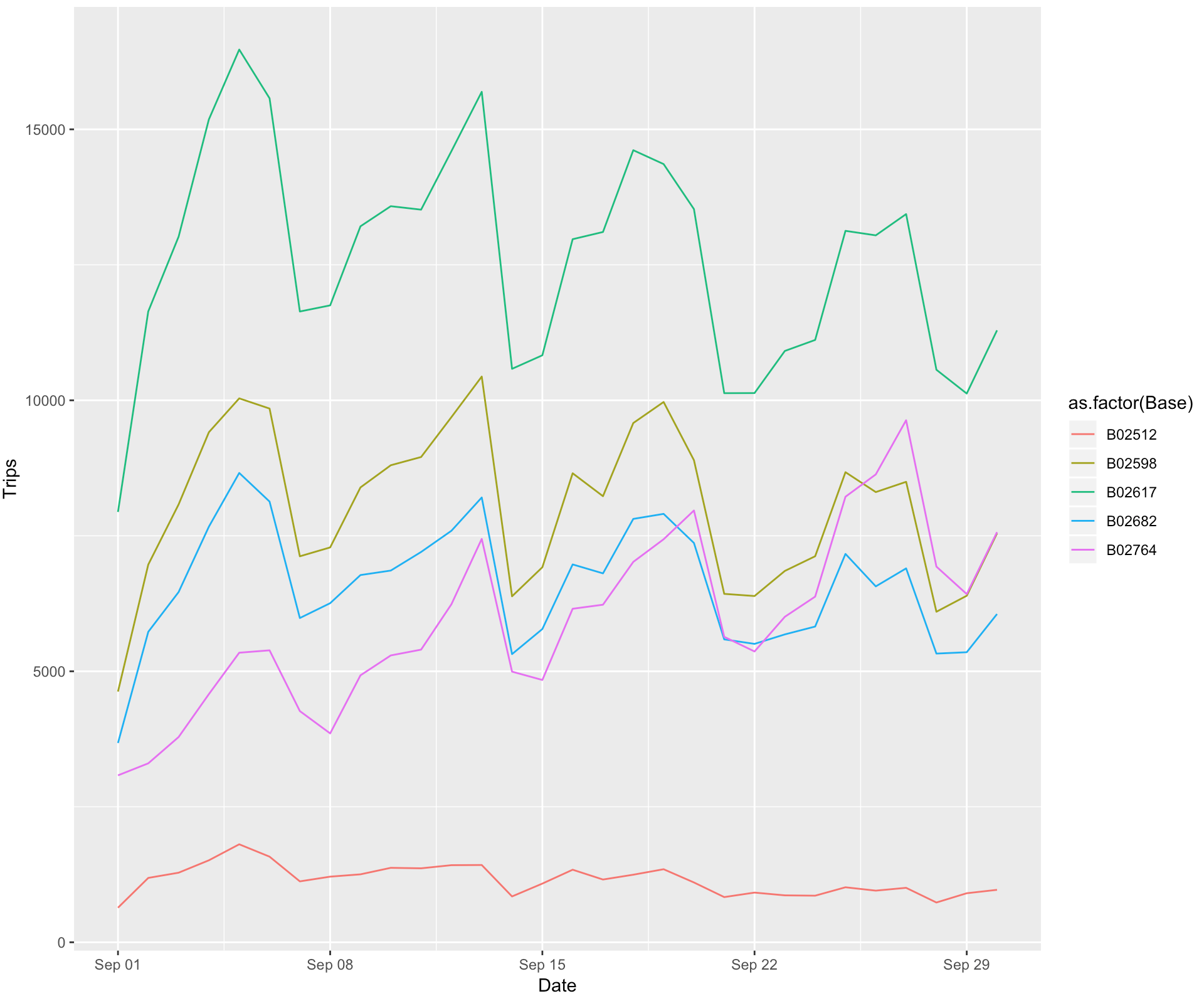
After all our hard work, we can finally graph our data!
ggplot(graph, aes(x = Date, y = Trips, color = as.factor(Base))) + geom_line()